Tuesday, August 7, 2018

GIS Programming Module 11

This post will focus on thing I have learned over the course of the semester in GIS Programming this year. The final Module focused on sharing tools. In the example above we took a tool and modified it so that we could share it either on networks or as a compressed .zip file.

1. First the fact that scripting can be used to run tools in ArcGIS blew my mind at first. Once we had a few lessons on the topic I was able to pick up the steps and recognize the scripting. It is actually a helpful way to run tool after tool without having to manipulate the feature classes in between.

2. This leads me to another thing I picked up along the course. At first I was overwhelmed when looking at certain scripts we were using for the lessons. As the class went on I was able to pick up the language much quicker and slowly, but surely understand the goal of the script. One day a commercial came on during a break in my favorite TV show (That 70’s Show). There was a giant computer screen with coding on it and it was meant to seem as if someone was hacking a computer, but I actually could make out some of the code!! I felt proud that I was learning something new having to do with computer language.

3. Finally the inner workings of ArcGIS  have always fascinated me and in this course we have learned yet another amazing capability of this program that make it far more efficient and ground breaking.

Wednesday, August 1, 2018

GIS Programming Module 10

This week in the lab we worked with taking a completed script and turning it into a usable tool in ArcMap. We set certain parameters for the tool and adjusted the script to then pull from the user inputs to make it universal. See the parameter settings and results windows below along with the steps to creating a tool.
1. The first step is to create the toolbox shell in ArcCatalog

2. Next you create a script tool in the toolbox and attach your .py script to the tool. This gives the tool guidelines on how to run.

3. Next you set parameters for data entry. This will allow for a better user interface and correct data entry.

4. Finally adjust your script to accept the data entered by the user instead of hard set file paths.

5. Check your script tool to confirm the proper operation.


Thursday, July 26, 2018

GIS Programming Peer Review 2

Peer Review 2
The work I chose to review incorporates an original idea of finding a solution to a problem that will arise in the future with the inevitable eruption of Indonesian volcanoes. Bear-Crozier, Kartadinata, Heriwaseso, and Nielsen’s (2012) application involves a Python based script used to simplify the process of installing and running a core prediction model. The model allows for analysis and prediction of volcanic ash fall following an eruption. The product was developed in cooperation with three major GIS agencies
The paper makes a strong case for the need for the solution. The hazards are clearly explained and show with an example how the research will help scientists predict the ash flow of future eruptions in the Indonesian region. The example itself is a great strength of the research showing that the developed script is in fact executable and provides valid analysis tools for scientists to use when studying the region. In the event that a volcanic natural disaster occurs in the region products will be available to provide the necessary evacuations and notifications. This was not possible with the previous data and models provided.
            One of the few weaknesses of the research is the usage of acronyms. The effort improves as the reader continues through the document, but at the beginning there are a few instances of acronyms being used that are research specific and everyday users would not understand the meaning. Descriptions are provided later in the body of the paper, but few instances at the start could leave the readers confused as to what is being discussed. This is only a minor readability flaw and would not affect the overall understanding of the research. The only other weakness I discovered is the fact that there is no new science developed in the research. The paper definitely describes a solution to a problem, but the solution is a Python based script that simplifies installation and running of a core model. There is definitely science involved in the programming of the package for running the core model (FALL3D). The script that the team developed is simply an adaptation that will make the process of volcanic ash fall analysis more streamlined. This is a weakness that does not take away from the research, but it does disqualify it as developmental in my opinion.
            The research is clearly laid out in chronological order how the study came about and who worked together to accomplish the results. The collaboration of three GIS departments shows the checks and validation that went on to achieve valuable and relevant results. If a single organization carried out the work then the results could be biased or not geared toward a universal solution. In this case the research methods are transparent and follow all scientific guidelines.
The single thing I liked most about the research is the use of illustrations. Being a visual learner the illustrations greatly increased my understanding of the study location and overall results of the research. There are many illustrations within the document that visually depict the processes and results of the study. The amount of illustrations is definitely a positive thing, but a few of the illustrations could have better labeling geared toward non-GIS familiar users. Some illustrations used an advanced or system specific labeling method that could make it confusing to some readers. I would have utilized a more “Plain English” approach to describing the technical illustrations.    
In wrapping up the study Bear-Crozier et al. (2012) conclude that the newly created process does in fact generate a usable product and proves the point with an example. I find this to be very important to the work because it shows the success of the research and how the accomplishments work in the analysis of future eruptions.

References
Bear-Crozier, A. N., Kartadinata, N., Heriwaseso, A., & Nielsen, O. (n.d.). Development of python-FALL3D: A modified procedure for modelling volcanic ash dispersal in the Asia-Pacific region (2012 ed., Vol. 64, Nat Hazards, pp. 821-838, Publication). doi:10.1007/s11069-012-0273-7

Monday, July 23, 2018

GIS Programming Module 9

This week in the lab we worked with Raster and Python scripting. It is really quite interesting how easily you can manipulate raster data with simple code and produce a result that would take longer in my opinion using ArcMap. The following is a result of analysis from the lab that was carried out strictly through Python script.
For a little background we were able to carry out slope and aspect analysis to produce a raster with ideal areas (in green) that met our parameters.

Tuesday, July 17, 2018

GIS Programming Module 8

This week in the lab we practiced pulling data from shapefiles and writing it in .txt files on Notepad for example. The process also works in reverse where you can pull information from a .txt document and populate shapefile attribute data. The results are shown below. The goal was to pull attribute data out of a shapefile and print it into a .txt file in a configuration that was readable.
The following pseudocode was used to accomplish the process. I am not including the actual code for obvious reasons, but this should show the overarching thought process behind populating a .txt file from attribute data.
START
Modules and Classes imported
Workspace set
Overwrite settings changed to overwrite existing files
Working shapefile variable set
Search Cursor used to select FID, Shape, and NAME attributes
Text document created for data to be written in
Iteration through rows started
    Vertex variable created, set to 0
    Iteration through arrays and points started
          Vertex variable changed to add 1
          Variable created as a string of text to write to file
                Result printed in Interactive window to error check
                Data written to .txt file
Text file closed
Variables row and cursor are deleted
END

Wednesday, July 11, 2018

GIS Programming Module 7

This assignment had some difficult steps and some that were fairly simple. The biggest issue I had with the assignment was the instructions outlined by steps. Some had excellent instructions on how to accomplish each step while others simply offered a solution, but did not really explain how the solution would work to accomplish the task. For example adding the variables from the cursor to the newly created dictionary threw me for a loop (pun intended). I spent two days trying to figure this out. Finally I reverted back to working with lists and for loops and realized the step was far simpler than I originally thought. The only other issue I had when working with the script was figuring out how the assignment wanted the results displayed on the window. Spaces or no spaces? Message data or not and for which steps? I understand the goal is to get us to work with the scripts and accomplish different tasks for different steps, but the instructions for the results display were set in different locations on the assignment and it took reading the document multiple times and re-scripting to come to a sensible conclusion that still could be interpreted as incorrect according to the instructions and example. A clearer reference should be used as to what result is required for steps 9-11.


Wednesday, June 27, 2018

GIS Programming Module 6

The process for writing the script was fairly simple for this lab with the help of the syntax helper tools. First I created the comments for the script with correct naming conventions and dates. Second I started with importing arcpy and environment modules and setting the workspace to my folder as well as allowing overwriting in the environment. Now it was time to start running the tools. First the AddXY tool gave me issues due to the fact that the tool alters the original shapefile by adding the XY data directly to those attributes. To fix this following the syntax helper I added a line of code to create a copy of the shapefile prior to adding the data. This allowed me to keep the original in my data folder. Next I added the code to create the correct 1000 meter buffer around the locations. This tool was fairly easy to code and ran perfectly the first time. Finally the dissolve tool gave me issues due to the fact that it was a management tool rather than an analysis tool. Since I had not used the tool many times in the application I incorrectly had it coded as an analysis tool (arcpy.Dissolve_analysis). As you can imagine the error code that was generated threw me for a loop. After a while of troubleshooting I realized the simple mistake and fixed the code allowing it to run properly.  To finish the code I added the print statements after all of the tools to print the correct data for the deliverable.

Tuesday, June 19, 2018

GIS Programming Module 5

This week in the lab we worked with creating Models and running scripts in ArcMap. To create the Model I completed the following steps.

1.       The first Step is to create a toolbox for the model to live in and set the workspace environment to the results folder for the module.
2.       Then the model is created and named appropriately

3.       For this model the input shapefiles were added by dragging directly from the ArcGIS table of Contents
4.       The tools, Clip, Select, and Erase were all added by dragging them into the window from the toolbox.
5.       Then the connections were made by filling each tool with the required parameters or shapefiles (inputs/outputs).
   6.       Finally the model was saved and exported to a script in a .py format.

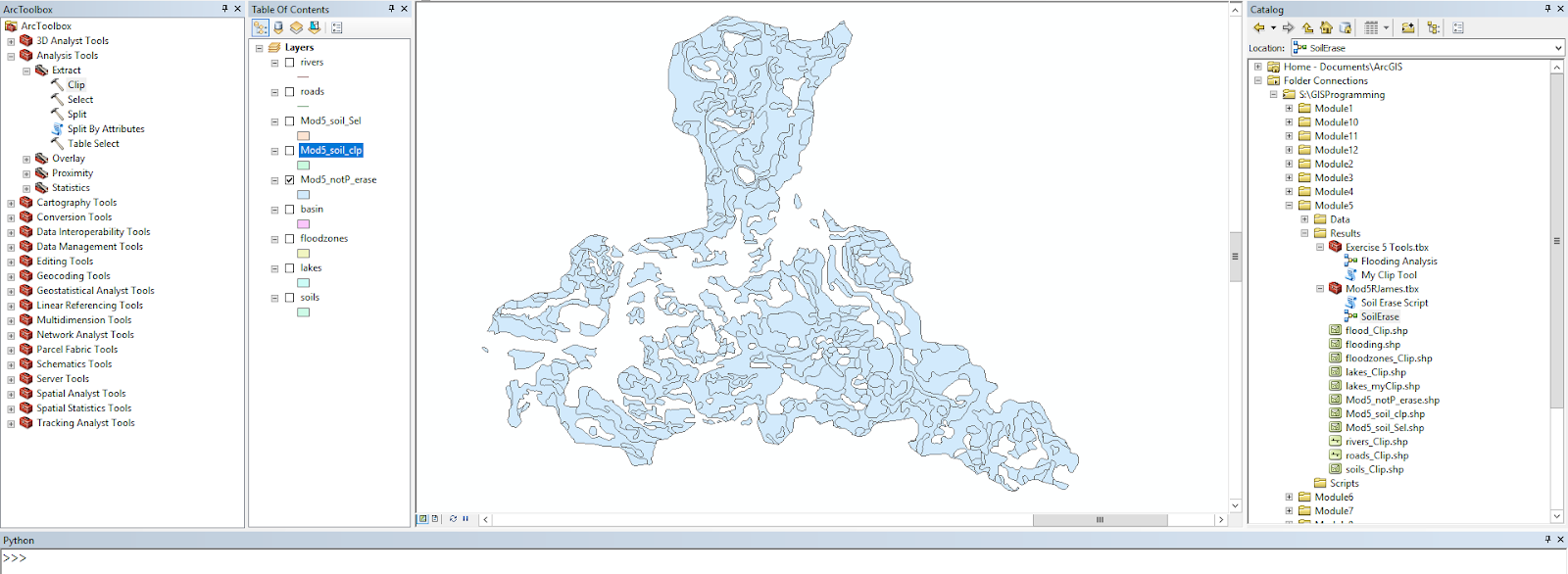
These steps resulted in the following flowchart and map results.


Wednesday, June 13, 2018

GIS Programming Peer Review 1

Link:
https://www-jstor-org.ezproxy.lib.uwf.edu/stable/42657268?Search=yes&resultItemClick=true&searchText=python&searchText=scripting&searchUri=%2Faction%2FdoBasicSearch%3FQuery%3Dpython%2Bscripting&refreqid=search%3A1ff09cdfb20ab992fb9dfb774319df52&seq=1#page_scan_tab_contents

The article I reviewed discusses the creation of a geoprocessing tool for ArcGIS using Python that simplifies a simulation procedure and automates the data flow between predictive models. The tool was created based on a need for less human interaction and error when using hydrodynamic and morphodynamic modelling of coastlines. In the study ArcGIS was chosen due to the ability to work with and analyze raster surface models and the scripting support provided through the Python scripting language.
The development of the tool seems to have stemmed from need for a solution to the problem of entering data manually and converting data between two different models. As described in the article this process when accomplished manually would be lengthy and riddled with human errors. The originality is shown in the BeachMM tool since it was created specifically to work with the two separate existing models for hydrodynamics.
Rather than a research paper, the article reads like an instruction manual for how the tool works with the two preexisting models. There is some history present about the previous models and why the research is taking place, but the focus of the paper is more of a how the tool was created and for what purpose rather than a step-by-step.
There are many strengths in the article. I believe the author clearly describes the need for the tool and how it will assist in the analysis process. There is also plenty of background information on the two preexisting models and how they are being used in the analysis of the coastal erosion. Overall the article is a strong presentation of how the tool was created and how it will be used in the analysis process.
Weaknesses of the article include the fact that the research is separate from the topic of the article. The research being done is on coastal erosion and the article focuses on the tool used to enhance the analysis process. In my opinion this article should be a section or chapter of a larger research project. There is still information on why the tool is being created, but the larger overarching research topic is lacking in description or background.
In the article the methods are clearly developed from inception of the idea to examples of the tool working with the preexisting models. The article leans toward the technical side, but provides a clear path to follow of how the tool was developed. One thing I really enjoyed about the article is the images of the analysis and actual desktop representations of the tool in action. This is extremely valuable for visual learner rather than two more pages of columned text.
The results of the development are clearly shown in the article and the references are well cited throughout the text and in the acknowledgements section. The article scores high in quality and quantity in my opinion seeing that it is only about nine pages and could realistically fill a chapter in the Esri ArcGIS manual for the tool with more explanation. The readability of the article ranked slightly lower in my opinion due to the highly technical nature of the topic. I understand that this class and topic are technical to begin with, but someone with no experience in GIS or coding would have a very hard time in deciphering some of the processes and steps of development.

References:

Silva, A. M., Almeida, Nobre, Taborda, R. P., & Matos. (2013). Integration of beach hydrodynamic and morphodynamic modelling in a GIS environment. Journal of Coastal Conservation, 17(2), 201-210. doi: https://www-jstor-org.ezproxy.lib.uwf.edu

GIS Programming Module 4


      In part one the script debugging gave me a lot of fits due to the small errors that I am not use to catching yet. Once I realized what they were the rest of the script debugging went pretty smooth. 


Adding the try-except statement was pretty much a copy paste from the exercise. The difficult part was setting a variable to catch the errors and print the actual error type rather than just the fact that there was an error. This was for part A. For Part B it was a little more challenging to figure out exactly what to do to make the script print the data. After I got it to work I realized it was a lot simpler than I thought, but going into the problem I didn’t know where to start. I entered the basic try-except statement, then played around with the printing after the except statement to attempt to get the data printed. This was the key. Once I was able to make something print I had the solution and was able to complete this part of the lab.

Tuesday, June 5, 2018

GIS Programming Module 3

This week in the lab we focused on error management and creating code from scratch. Below is my output and scripting to reach the goal of the lab.
To remove the numbers from the list that were equal to the “bad” number that was randomly generated I had to set a variable for how many bad numbers there were in the list. I then used a while loop when bad was greater than zero to remove one iteration of the number from the list and decrease the value of bad by one. This continued until bad equaled zero therefore removing all bad numbers from the list.

Monday, May 28, 2018

GIS Programming Module 2

This week the lab was focused on writing our own script to run in an attempt to print our last name with the amount of letters multiplied by 3. The following screenshot is the result I came up with without showing the whole script. When I started on the script I was a little unsure where to start off, but once you set a variable the rest flows fairly quickly. I would say most of this lab dealt with a logical flow to represent different numbers and text that the lab asked for. Some of the steps are sort of hidden when only looking at the result. On the screen shot you can only see the printed last name variable and triple count of the letters in the last name. 
The process involved a lot more than it seems. First a string was created with your full name, then a list followed by the names split into first, middle, last. From here you were able to select your last name and get a count that you then multiplied by three. The ending goal in the lab was not to simply make the script print what you want, but to make it universal so that you could simply change the full name in the first variable and the script would adjust and display the correct information for that particular name. It was an interesting lab that showed us a basic interface using python and I can't wait to continue with the scripting!

Monday, May 21, 2018

GIS Programming Module 1

For our first module in GIS Programming we were introduced to Python and scripting in ArcGIS. For this week we learned how to run a previously written script. The script created a foler for the class this semester and organized them into modules for each week and separate folders within each module for Data, Scripts, and Results each week.


The process to actually run the script in the PythonWin program was fairly simple. I chose the method of clicking on the Run button in the menu bar. After clicking on the button a window was opened that asked which script I wanted to run, if I had any arguments to add, and what debugging options I wanted. I confirmed the folder script was selected and the argument and debugging options were left at the default settings. Then a simple click on the “OK” button actually ran the script. After the scrip was run the window simply disappears and the script is still open in the script window.

Saturday, January 13, 2018

GIS Management Lab 1

This week in the Lab we focused on the introduction of GIS Management and worked with business processes and flowcharts. Two cases we studied used GIS in some way to better the business processes. This was our first attempt to identify the business processes and show how they changed so be gentle in the critique. The water service case study is definitely a business/single department based program that stayed within the departmental oversight environment. It focused on the field/mobile users which are the technicians utilizing the real time information. The bus location case study seems more project-based due to the fact that they are updating a previous system on the location app. This study falls under the “project” environment where the progress is monitored by team members. The study is focused on the casual/direct users that can pull up the information on the web based applications to located the buses. The following are the business process flow charts to compare before and after the changes.


References:
Croswell, P. L. (2009). The GIS Management Handbook. Frankfort, KY: Kessey Dewitt Publications.

Esri (2015). GIS Speeds Water Service Restoration. ArcNews Fall 2015 Vol., No. 3. 

Esri (2011). App Supplies Bus Locations and Schedules. ArcUser Fall 2011 

Sunday, December 10, 2017

Special Topics in GIS Lab 15

Dasymetric mapping is 

"a technique in which attribute data that is organized by a large or arbitrary area unit is more accurately distributed within that unit by the overlay of geographic boundaries that exclude, restrict, or confine the attribute in question. For example, a population attribute organized by census tract might be more accurately distributed by the overlay of water bodies, vacant land, and other land-use boundaries within which it is reasonable to infer that people do not live."

-https://support.esri.com/en/other-resources/gis-dictionary/term/dasymetric%20mapping

For the lab this week we focused on dasymetric mapping and I found this definition from esri helpful so I wanted to add it here. This week really focused a lot on basic arcGIS skills with an in depth understanding of how populations are distributed. For the lab we used a raster product of population density or imperviousness to get more accurate estimates for populations in certain areas.

This image is a layout of the census tracts used for the population clipped and erased to remove hydrology features. It is overlayed on the raster of imperviousness to show the population densities. This product along with many statistical editing allowed us to calculate more accurate population estimates.

Tuesday, December 5, 2017

Special Topics in GIS Lab 14

This week in the lab we focused on the topic of Gerrymandering which is the representation of of a population through skewed congressional districts. We looked at metrics that could be used to measure the skewness of the districts. The two metrics used were compactness and community. Compactness measured how spread out and unnatural the district's shape was while community measured how many counties the district overlapped either completely or partially. For compactness the equation 400pi(area)/(perimeter)^2  can be used to get a value. This equation produces a result from 0-100 where 100 is the best compactness (a circle). The lowest compactness or 0 would be the worst case where the perimeter is very large and the area very small. For community the measurements were derived from running an intersect to see how many counties were divided into sections by the districts spatially and how many counties were included in each district total. Then the total divided counties were divided by the total counties within the districts to display a percentage of counties divided. Below are some examples of worst compactness and community scores. The first demonstrates low compactness and the second low community.


Wednesday, November 29, 2017

Special Topics in GIS Lab 13

This week in the lab we worked with scale and resolution. The lab focused on differences between line and polygon features in the first half and raster DEMs in the second portion described below.

To compare the two DEMs I focused on slope, aspect, and overall elevation. First the slopes of each DEM were mapped and the averages compared. Then for further analysis the slope maps were combined to display the slope difference between the two DEMs. Second the aspect of each DEM was mapped and compared to analyze the slope direction and general direction the terrain was facing. This analysis gave more of a horizontal representation of the differences rather than strictly elevation differences. Finally the overall elevation was compared for the two DEMs. The standard statistics were calculated and compared to determine the data represented.


The results clearly show that there is a difference between the SRTM and LiDAR data. Both of the DEMs were analyzed at 90m resolution. The slope of the separate DEMs seemed to follow the terrain feature of the area which was a drainage. The LiDAR model had a steeper average slope which revealed itself in the higher elevations of the terrain feature. The slope difference between the models is also shown in the visual. The areas where the slope is the steepest between the valleys and ridges tended to have a larger difference while relatively flat areas had a smaller difference.
              
The aspect maps of the DEMs at 90m resolution were fairly similar. The aspect analysis was meant to look at the models horizontal of directional facing representations rather than elevation. The results show that even though he models a very close match there are still some areas that have different aspects. This shows that the slopes differed between the certain areas enough to cause the software to display a different facing direction for the certain area. The differences are slight and nowhere near opposite direction, but if an accurate representation is vital then consideration should be taken in which model to use for a study.

Finally the elevation of the two models differs. In the table the results show that the LiDAR model has a lower average elevation along with a higher maximum and lower minimum elevation. To me these results show the LiDAR model as more complete. In the elevation comparison map the areas of largest elevation difference follow the trend in the slope difference map. They are in the specific areas of the terrain feature where the valley is transitioning to a ridge and has a steeper slope. The one interesting result is that the large differences in elevations are only seen on the southern side of the drainage in areas with steep slopes. The norther side of the terrain feature shows smaller differences between the two elevation models. This could be due to the location of the sensor platforms when the separate model’s data was collected.


The creation of the LiDAR and SRTM both involve air/space borne sensors. LiDAR can also be collected with ground based sensors, but larger areas tend to be collected on using airborne sensors. These two sensors are both collecting elevation data, but one is tens to hundreds of miles in the air, while the other is less than a mile above the ground. The fact that the SRTM data is at 90m is impressive considering how high up in space the sensor is located. Overall I would have to say that the LiDAR model is a more accurate representation of the drainage feature in all perameters due to the fact that the sensor is collecting data far closer to the source, the model was derived from a higher resolution product, and the LiDAR sensor was probably built for high resolution large scale ground mapping.

Wednesday, November 22, 2017

Special Topics in GIS Lab 12

This week in the lab we focused on Graphically Weighted Regression or (GWR). This type of regression analysis uses the same analysis as the OLS, but takes into account a spacial aspect. For the lab this week we used a county area with locations and types of different crimes. The goal was to select a particular dependent variable and figure out which independent variables are able to describe the dependent variable the best. Using techniques learned from previous labs I created a correlation matrix and exploratory regression in ArcGIS to determine the most descriptive regression was completed using three distinct independent variables. I then used these variables to create an OLS and GWR analysis for comparison. After reviewing the results it was clear that the GWR was more than 10% more accurate in describing the dependent variable than the OLS. This is due to the GWR using the spatial aspect rather than analyzing as a whole.

Monday, November 13, 2017

Special Topics in GIS Lab 11

Using regression analysis in ArcGIS this week was eye opening. Prior to this week the analysis was all done in Excel and displayed in spreadsheets. This week we were able to pull the information into ArcGIS and perform the same analysis in a way that produced a visual representation as well as a summary of statistical reports that help the user analyse the testing. First you need the data for the analysis to be performed on. Then you simply use the Ordinary Least Squares tool in ArcGIS to set your data set, dependent, and independent variable(s) and let the program do the work. The results are provided in an easy to read report that gives all the information you need to decide if the results fit your analytical needs. This week in the lab we worked on interpreting the results. The focus was on the many values that the program calculates to analyse the regression. The tool that you run in ArcGIS even incorporated instructions int he results for reading the reported variables and determining if the result is what you are looking for.

The output of the OLS tool produces a residual map that visually shows the difference the actual data is from an expected value on the regression line. This visual aid can help us determine the accuracy and bias that could be present in the results. For instance if there is a pattern in the results or areas where the residuals are similar in a certain area it could show a bias or non-random correlation. This information is good to have because it could clue you into the fact that you need to use another variable to run the regression analysis.

Finally at the end of the lab (of course) it was revealed that rather than running the tool many times on different independent variables you can simply run another tool that includes all of the variables you wish to analyse and reports the most accurate result possible. The capability of technology today is impressive and makes me wonder what the engineers and analysts will have the software calculating for us next!

Monday, November 6, 2017

Special Topics in GIS Lab 10

The lab this week focused on regression and how to analyze data to determine predicted values. The focus this week was in Microsoft Excel rather than ArcGIS. The analysis was formula intensive, but allowed for a better understanding of how to use Excel to gather the data parameters you want for analysis. The Excel program also has a great tool that can be used to accomplish the majority of the regression analysis in one easy step.
This example sums up the processes we used in Excel this week. The goal is to determine if the data points you collect or are given have any correlation and if so how well are the values predictors for each other. In our example two stations reported rainfall annually for a given number of years. One station failed to report for a span of years and it is your job to predict the missing amounts to complete the dataset. In order to do that you perform a regression analysis on the rest of the data to find the slope and intercept value of a "trendline" for the data. This line equation can then be used to enter your x-values from one station and find our y-values for the missing station numbers. The values will not be perfect, but they will be predictions in line with the rest of the data.