Special Topics in GIS Lab 15

Dasymetric mapping is 

"a technique in which attribute data that is organized by a large or arbitrary area unit is more accurately distributed within that unit by the overlay of geographic boundaries that exclude, restrict, or confine the attribute in question. For example, a population attribute organized by census tract might be more accurately distributed by the overlay of water bodies, vacant land, and other land-use boundaries within which it is reasonable to infer that people do not live."

-https://support.esri.com/en/other-resources/gis-dictionary/term/dasymetric%20mapping

For the lab this week we focused on dasymetric mapping and I found this definition from esri helpful so I wanted to add it here. This week really focused a lot on basic arcGIS skills with an in depth understanding of how populations are distributed. For the lab we used a raster product of population density or imperviousness to get more accurate estimates for populations in certain areas.

This image is a layout of the census tracts used for the population clipped and erased to remove hydrology features. It is overlayed on the raster of imperviousness to show the population densities. This product along with many statistical editing allowed us to calculate more accurate population estimates.

Special Topics in GIS Lab 14

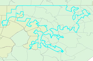
This week in the lab we focused on the topic of Gerrymandering which is the representation of of a population through skewed congressional districts. We looked at metrics that could be used to measure the skewness of the districts. The two metrics used were compactness and community. Compactness measured how spread out and unnatural the district's shape was while community measured how many counties the district overlapped either completely or partially. For compactness the equation 400pi(area)/(perimeter)^2  can be used to get a value. This equation produces a result from 0-100 where 100 is the best compactness (a circle). The lowest compactness or 0 would be the worst case where the perimeter is very large and the area very small. For community the measurements were derived from running an intersect to see how many counties were divided into sections by the districts spatially and how many counties were included in each district total. Then the total divided counties were divided by the total counties within the districts to display a percentage of counties divided. Below are some examples of worst compactness and community scores. The first demonstrates low compactness and the second low community.